GIS mit ggplot2
GIS mit ggplot2
Die Ausgangssituation sei ein File mit Sammelpunkten und Angaben zu Datenquelle und per Sequenz bestimmtem Genotyp.
							> read.csv('https://lehre.cos.uni-heidelberg.de/presentations/open/R/downloads/
								cbpoints.csv') -> pts
							> head(pts, 3)
						  X SequenceType     Lat    Long DataSource
						1 1            1 51.2446  9.2932        PCR
						2 2           3A 40.9154 40.9154        PCR
						3 3            1 55.6875  9.8683        PCR
Das Ziel ist die Visualisierung dieser Daten auf einer Europa-Karte.
GIS mit ggplot2
Folgende R-Pakete werden gebraucht:
						# install.packages(c('sf','ggplot2','rnaturalearth','rnaturalearthhires','rnaturalearthdata'))
						library('sf')
						library('ggplot2')
						library('rnaturalearth')
						library('rnaturalearthhires')
						library('rnaturalearthdata')
GIS mit ggplot2
Wir brauchen ein SF-Object mit Geo-Daten:
						ptsf <- st_as_sf(pts, coords=c('Long', 'Lat'))
						Fehler in st_as_sf.data.frame(pts, coords = c("Long", "Lat")) :
						missing values in coordinates not allowed
						# Ups
						...
						105 105            1 49.69232 22.4858833        PCR
						106  NA                    NA         NA        PCR
						107 107            1 39.80000 21.1166667        PCR
						...
						#Aha...
						> pts <- pts[!is.na(pts$Lat),]
						> ptsf <- st_as_sf(pts, coords=c('Long', 'Lat'))
						> sf_use_s2(FALSE) # S2 features abschalten
						> st_crs(ptsf) = 4326 # Projektion setzen
GIS mit ggplot2
						> ptsf
						Simple feature collection with 199 features and 3 fields
						Geometry type: POINT
						Dimension:     XY
						Bounding box:  xmin: -3.220519 ymin: 36.23028 xmax: 82.53025 ymax: 62.92458
						Geodetic CRS:  WGS 84
						First 10 features:
						    X SequenceType DataSource                geometry
						1   1            1        PCR  POINT (9.2932 51.2446)
						2   2           3A        PCR POINT (40.9154 40.9154)
						3   3            1        PCR  POINT (9.8683 55.6875)
						4   4            1        PCR   POINT (14.65 58.3333)
						5   5           3A        PCR POINT (28.9889 41.1836)
						...
Punkte sind vorbereitet.
GIS mit ggplot2
Dann brauchen wir noch eine Karte.
						eu <- c("Albania","Austria","Belgium","Bulgaria","Belarus","Bosnia and Herzegovina","Croatia","Cyprus",
        					"Czech Republic","Denmark","Estonia","Finland","France",
        					"Germany","Greece","Hungary","Ireland","Italy","Latvia",
        					"Lithuania","Luxembourg","Macedonia","Malta","Moldova","Montenegro","Netherlands","Poland",
        					"Portugal","Romania","Russia","Slovakia","Republic of Serbia","Slovenia","Spain",
        					"Sweden","Switzerland","United Kingdom","Ukraine")
						euro <- ne_states(country=eu, returnclass = "sf")
						w <- ggplot() + geom_sf(data=euro_cropped, col="darkgrey", show.legend=F)
						w
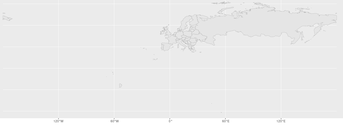
GIS mit ggplot2
Nicht schön, als Europakarte, besser zuschneiden.
						euro <- ne_countries(scale = "medium", returnclass = "sf")
						euro_cropped <- st_crop(euro, xmin = -20, xmax = 45, ymin = 30, ymax = 73)
						ptsf_cropped <- st_crop(ptsf, xmin = -20, xmax = 45, ymin = 30, ymax = 73)
						w <- ggplot() + geom_sf(data=euro_cropped, col="darkgrey", show.legend=F)
						w
GIS mit ggplot2
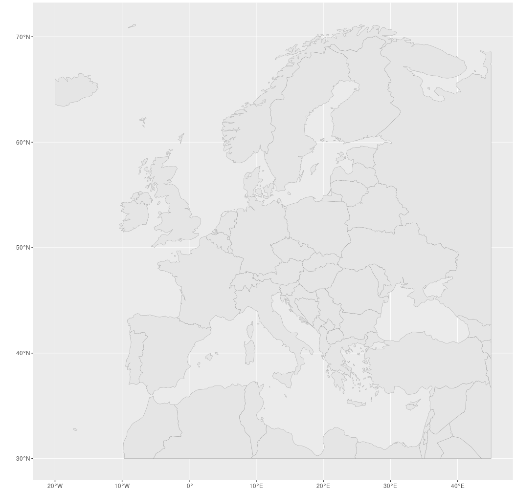
Besser.
GIS mit ggplot2
Fehlen noch die Punkte.
						w <- w + geom_sf(data=ptsf_cropped,
							aes(shape=ptsf_cropped$DataSource,col=ptsf_cropped$SequenceType),
							show.legend=T)
						w
GIS mit ggplot2
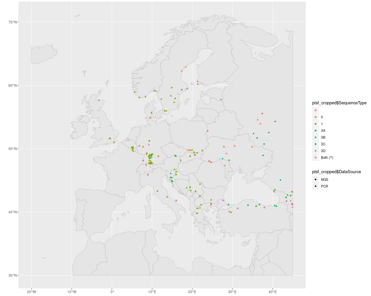
Datenquelle als Form, Sequenztyp als Farbe visualisiert.(Mission accomplished...)
Übungen